criterion: Robust, reliable performance measurement and analysis
This library provides a powerful but simple way to measure software performance. It consists of both a framework for executing and analysing benchmarks and a set of driver functions that makes it easy to build and run benchmarks, and to analyse their results.
The fastest way to get started is to read the online tutorial, followed by the documentation and examples in the Criterion.Main module.
[Skip to Readme]


Modules
[Index] [Quick Jump]
Flags
Manual Flags
| Name | Description | Default |
|---|---|---|
| fast | compile without optimizations | Disabled |
| embed-data-files | Embed the data files in the binary for a relocatable executable. (Warning: This will increase the executable size significantly.) | Disabled |
Use -f <flag> to enable a flag, or -f -<flag> to disable that flag. More info
Downloads
- criterion-1.6.4.1.tar.gz [browse] (Cabal source package)
- Package description (as included in the package)
Maintainer's Corner
For package maintainers and hackage trustees
Candidates
- No Candidates
| Versions [RSS] | 0.1, 0.1.2, 0.1.3, 0.1.4, 0.2.0, 0.3.0, 0.4.0, 0.4.1.0, 0.5.0.0, 0.5.0.1, 0.5.0.2, 0.5.0.3, 0.5.0.4, 0.5.0.5, 0.5.0.7, 0.5.0.8, 0.5.0.9, 0.5.0.10, 0.5.1.0, 0.5.1.1, 0.6.0.0, 0.6.0.1, 0.6.1.1, 0.6.2.0, 0.6.2.1, 0.8.0.0, 0.8.0.1, 0.8.0.2, 0.8.1.0, 1.0.0.0, 1.0.0.1, 1.0.0.2, 1.0.1.0, 1.0.2.0, 1.1.0.0, 1.1.1.0, 1.1.4.0, 1.2.0.0, 1.2.1.0, 1.2.2.0, 1.2.3.0, 1.2.4.0, 1.2.5.0, 1.2.6.0, 1.3.0.0, 1.4.0.0, 1.4.1.0, 1.5.0.0, 1.5.1.0, 1.5.2.0, 1.5.3.0, 1.5.4.0, 1.5.5.0, 1.5.6.0, 1.5.6.1, 1.5.6.2, 1.5.7.0, 1.5.8.0, 1.5.9.0, 1.5.10.0, 1.5.11.0, 1.5.12.0, 1.5.13.0, 1.6.0.0, 1.6.1.0, 1.6.2.0, 1.6.3.0, 1.6.4.0, 1.6.4.1 (info) |
|---|---|
| Change log | changelog.md |
| Dependencies | aeson (>=2 && <2.3), base (>=4.9 && <5), base-compat-batteries (>=0.10 && <0.15), binary (>=0.8.3.0), binary-orphans (>=1.0.1 && <1.1), bytestring (>=0.10.8.1 && <1.0), cassava (>=0.3.0.0), code-page, containers, criterion, criterion-measurement (>=0.2 && <0.3), deepseq (>=1.1.0.0), directory, exceptions (>=0.8.2 && <0.11), filepath, Glob (>=0.7.2), js-chart (>=2.9.4 && <3), microstache (>=1.0.1 && <1.1), mtl (>=2), mwc-random (>=0.8.0.3), optparse-applicative (>=0.18 && <0.20), parsec (>=3.1.0), prettyprinter (>=1.7 && <1.8), prettyprinter-ansi-terminal (>=1.1 && <1.2), statistics (>=0.14 && <0.17), text (>=0.11), time, transformers, transformers-compat (>=0.6.4), vector (>=0.7.1), vector-algorithms (>=0.4) [details] |
| Tested with | ghc ==8.0.2, ghc ==8.2.2, ghc ==8.4.4, ghc ==8.6.5, ghc ==8.8.4, ghc ==8.10.7, ghc ==9.0.2, ghc ==9.2.8, ghc ==9.4.8, ghc ==9.6.7, ghc ==9.8.4, ghc ==9.10.2, ghc ==9.12.2 |
| License | BSD-3-Clause |
| Copyright | 2009-present Bryan O'Sullivan and others |
| Author | Bryan O'Sullivan <bos@serpentine.com> |
| Maintainer | Ryan Scott <ryan.gl.scott@gmail.com> |
| Category | Development, Performance, Testing, Benchmarking |
| Home page | https://github.com/haskell/criterion |
| Bug tracker | https://github.com/haskell/criterion/issues |
| Source repo | head: git clone https://github.com/haskell/criterion.git |
| Uploaded | by ryanglscott at 2025-09-06T22:52:30Z |
| Distributions | Arch:1.6.3.0, Debian:1.5.6.2, Fedora:1.6.4.0, FreeBSD:1.1.0.0, LTSHaskell:1.6.4.0, NixOS:1.6.4.0, Stackage:1.6.4.1, openSUSE:1.6.4.0 |
| Reverse Dependencies | 28 direct, 3695 indirect [details] |
| Executables | criterion-report |
| Downloads | 126290 total (129 in the last 30 days) |
| Rating | 2.75 (votes: 8) [estimated by Bayesian average] |
| Your Rating | |
| Status | Docs available [build log] Last success reported on 2025-09-07 [all 1 reports] |
Readme for criterion-1.6.4.1
[back to package description]Criterion: robust, reliable performance measurement

![]()
criterion is a library that makes accurate microbenchmarking in
Haskell easy.
Features
-
The simple API hides a lot of automation and details that you shouldn't need to worry about.
-
Sophisticated, high-resolution analysis which can accurately measure operations that run in as little as a few hundred picoseconds.
-
Output to active HTML (with JavaScript charts), CSV, and JSON. Write your own report templates to customize exactly how your results are presented.
-
Linear regression model that allows measuring the effects of garbage collection and other factors.
-
Measurements are cross-validated to ensure that sources of significant noise (usually other activity on the system) can be identified.
To get started, read the tutorial below, and take a look at the programs in the examples directory.
Credits and contacts
This library is written by Bryan O'Sullivan (bos@serpentine.com) and maintained by Ryan Scott (ryan.gl.scott@gmail.com). Please report bugs via the GitHub issue tracker.
Tutorial
Getting started
Here's Fibber.hs: a simple and complete benchmark, measuring the performance of
the ever-ridiculous fib function.
{- cabal:
build-depends: base, criterion
-}

import Criterion.Main

-- The function we're benchmarking.
fib :: Int -> Int
fib m | m < 0     = error "negative!"
      | otherwise = go m
  where
    go 0 = 0
    go 1 = 1
    go n = go (n - 1) + go (n - 2)

-- Our benchmark harness.
main = defaultMain [
  bgroup "fib" [ bench "1"  $ whnf fib 1
               , bench "5"  $ whnf fib 5
               , bench "9"  $ whnf fib 9
               , bench "11" $ whnf fib 11
               ]
  ]
The
defaultMain
function takes a list of
Benchmark
values, each of which describes a function to benchmark. (We'll come
back to bench and whnf shortly, don't worry.)
To maximise our convenience, defaultMain will parse command line
arguments and then run any benchmarks we ask. Let's run our benchmark
program (it might take some time if you never used Criterion before, since
the library has to be downloaded and compiled).
$ cabal run Fibber.hs
benchmarking fib/1
time                 13.77 ns   (13.49 ns .. 14.07 ns)
                     0.998 R²   (0.997 R² .. 1.000 R²)
mean                 13.56 ns   (13.49 ns .. 13.70 ns)
std dev              305.1 ps   (64.14 ps .. 532.5 ps)
variance introduced by outliers: 36% (moderately inflated)

benchmarking fib/5
time                 173.9 ns   (172.8 ns .. 175.6 ns)
                     1.000 R²   (0.999 R² .. 1.000 R²)
mean                 173.8 ns   (173.1 ns .. 175.4 ns)
std dev              3.149 ns   (1.842 ns .. 5.954 ns)
variance introduced by outliers: 23% (moderately inflated)

benchmarking fib/9
time                 1.219 μs   (1.214 μs .. 1.228 μs)
                     1.000 R²   (1.000 R² .. 1.000 R²)
mean                 1.219 μs   (1.216 μs .. 1.223 μs)
std dev              12.43 ns   (9.907 ns .. 17.29 ns)

benchmarking fib/11
time                 3.253 μs   (3.246 μs .. 3.260 μs)
                     1.000 R²   (1.000 R² .. 1.000 R²)
mean                 3.248 μs   (3.243 μs .. 3.254 μs)
std dev              18.94 ns   (16.57 ns .. 21.95 ns)
Even better, the --output option directs our program to write a
report to the file fibber.html.
$ cabal run Fibber.hs -- --output fibber.html
...similar output as before...
Click on the image to see a complete report. If you mouse over the data points in the charts, you'll see that they are live, giving additional information about what's being displayed.
Understanding charts
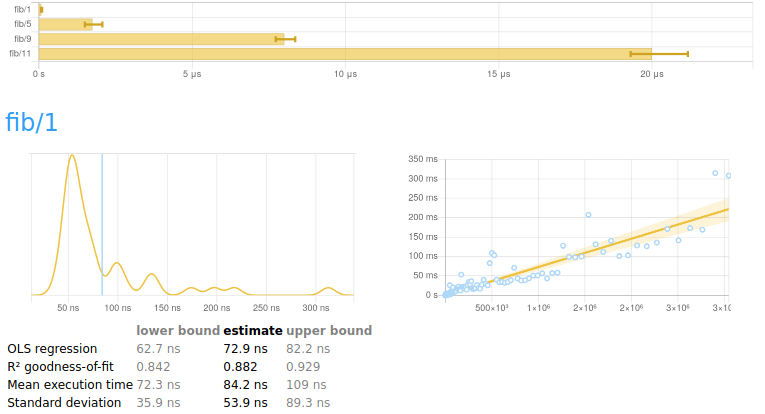
A report begins with a summary of all the numbers measured. Underneath is a breakdown of every benchmark, each with two charts and some explanation.
The chart on the left is a kernel density estimate (also known as a KDE) of time measurements. This graphs the probability of any given time measurement occurring. A spike indicates that a measurement of a particular time occurred; its height indicates how often that measurement was repeated.
[!NOTE] Why not use a histogram?
A more popular alternative to the KDE for this kind of display is the histogram. Why do we use a KDE instead? In order to get good information out of a histogram, you have to choose a suitable bin size. This is a fiddly manual task. In contrast, a KDE is likely to be informative immediately, with no configuration required.
The chart on the right contains the raw measurements from which the kernel density estimate was built. The \(x\) axis indicates the number of loop iterations, while the \(y\) axis shows measured execution time for the given number of iterations. The line “behind” the values is a linear regression generated from this data. Ideally, all measurements will be on (or very near) this line.
Understanding the data under a chart
Underneath the chart for each benchmark is a small table of information that looks like this.
| lower bound | estimate | upper bound | |
|---|---|---|---|
| OLS regression | 31.0 ms | 37.4 ms | 42.9 ms |
| R² goodness-of-fit | 0.887 | 0.942 | 0.994 |
| Mean execution time | 34.8 ms | 37.0 ms | 43.1 ms |
| Standard deviation | 2.11 ms | 6.49 ms | 11.0 ms |
The second row is the result of a linear regression run on the measurements displayed in the right-hand chart.
-
“OLS regression” estimates the time needed for a single execution of the activity being benchmarked, using an ordinary least-squares regression model. This number should be similar to the “mean execution time” row a couple of rows beneath. The OLS estimate is usually more accurate than the mean, as it more effectively eliminates measurement overhead and other constant factors.
-
“R² goodness-of-fit” is a measure of how accurately the linear regression model fits the observed measurements. If the measurements are not too noisy, R² should lie between 0.99 and 1, indicating an excellent fit. If the number is below 0.99, something is confounding the accuracy of the linear model. A value below 0.9 is outright worrisome.
-
“Mean execution time” and “Standard deviation” are statistics calculated (more or less) from execution time divided by number of iterations.
On either side of the main column of values are greyed-out lower and upper bounds. These measure the accuracy of the main estimate using a statistical technique called bootstrapping. This tells us that when randomly resampling the data, 95% of estimates fell within between the lower and upper bounds. When the main estimate is of good quality, the lower and upper bounds will be close to its value.
Reading command line output
Before you look at HTML reports, you'll probably start by inspecting the report that criterion prints in your terminal window.
benchmarking ByteString/HashMap/random
time                 4.046 ms   (4.020 ms .. 4.072 ms)
                     1.000 R²   (1.000 R² .. 1.000 R²)
mean                 4.017 ms   (4.010 ms .. 4.027 ms)
std dev              27.12 μs   (20.45 μs .. 38.17 μs)
The first column is a name; the second is an estimate. The third and fourth, in parentheses, are the 95% lower and upper bounds on the estimate.
-
timecorresponds to the “OLS regression” field in the HTML table above. -
R²is the goodness-of-fit metric fortime. -
meanandstd devhave the same meanings as “Mean execution time” and “Standard deviation” in the HTML table.
How to write a benchmark suite
A criterion benchmark suite consists of a series of
Benchmark
values.
main = defaultMain [
  bgroup "fib" [ bench "1"  $ whnf fib 1
               , bench "5"  $ whnf fib 5
               , bench "9"  $ whnf fib 9
               , bench "11" $ whnf fib 11
               ]
  ]
We group related benchmarks together using the
bgroup
function. Its first argument is a name for the group of benchmarks.
bgroup :: String -> [Benchmark] -> Benchmark
All the magic happens with the
bench
function. The first argument to bench is a name that describes the
activity we're benchmarking.
bench :: String -> Benchmarkable -> Benchmark
bench = Benchmark
The
Benchmarkable
type is a container for code that can be benchmarked.
By default, criterion allows two kinds of code to be benchmarked.
-
Any
IOaction can be benchmarked directly. -
With a little trickery, we can benchmark pure functions.
Benchmarking an IO action
This function shows how we can benchmark an IO action.
import Criterion.Main

main = defaultMain [
    bench "readFile" $ nfIO (readFile "GoodReadFile.hs")
  ]
We use
nfIO
to specify that after we run the IO action, its result must be
evaluated to normal form, i.e. so that
all of its internal constructors are fully evaluated, and it contains
no thunks.
nfIO :: NFData a => IO a -> Benchmarkable
Rules of thumb for when to use nfIO:
-
Any time that lazy I/O is involved, use
nfIOto avoid resource leaks. -
If you're not sure how much evaluation will have been performed on the result of an action, use
nfIOto be certain that it's fully evaluated.
IO and seq
In addition to nfIO, criterion provides a
whnfIO
function that evaluates the result of an action only deep enough for
the outermost constructor to be known (using seq). This is known as
weak head normal form (WHNF).
whnfIO :: IO a -> Benchmarkable
This function is useful if your IO action returns a simple value
like an Int, or something more complex like a
Map
where evaluating the outermost constructor will do “enough work”.
Be careful with lazy I/O!
Experienced Haskell programmers don't use lazy I/O very often, and here's an example of why: if you try to run the benchmark below, it will probably crash.
import Criterion.Main

main = defaultMain [
    bench "whnfIO readFile" $ whnfIO (readFile "BadReadFile.hs")
  ]
The reason for the crash is that readFile reads the contents of a
file lazily: it can't close the file handle until whoever opened the
file reads the whole thing. Since whnfIO only evaluates the very
first constructor after the file is opened, the benchmarking loop
causes a large number of open files to accumulate, until the
inevitable occurs:
$ ./BadReadFile
benchmarking whnfIO readFile
openFile: resource exhausted (Too many open files)
Beware “pretend” I/O!
GHC is an aggressive compiler. If you have an IO action that
doesn't really interact with the outside world, and it has just the
right structure, GHC may notice that a substantial amount of its
computation can be memoised via “let-floating”.
There exists a somewhat contrived example of this problem, where the first two benchmarks run between 40 and 40,000 times faster than they “should”.
As always, if you see numbers that look wildly out of whack, you shouldn't rejoice that you have magically achieved fast performance—be skeptical and investigate!
[!TIP] Defeating let-floating
Fortunately for this particular misbehaving benchmark suite, GHC has an option named
-fno-full-lazinessthat will turn off let-floating and restore the first two benchmarks to performing in line with the second two.You should not react by simply throwing
-fno-full-lazinessinto every GHC-and-criterion command line, as let-floating helps with performance more often than it hurts with benchmarking.
Benchmarking pure functions
Lazy evaluation makes it tricky to benchmark pure code. If we tried to saturate a function with all of its arguments and evaluate it repeatedly, laziness would ensure that we'd only do “real work” the first time through our benchmarking loop. The expression would be overwritten with that result, and no further work would happen on subsequent loops through our benchmarking harness.
We can defeat laziness by benchmarking an unsaturated function—one that has been given all but one of its arguments.
This is why the
nf
function accepts two arguments: the first is the almost-saturated
function we want to benchmark, and the second is the final argument to
give it.
nf :: NFData b => (a -> b) -> a -> Benchmarkable
As the
NFData
constraint suggests, nf applies the argument to the function, then
evaluates the result to normal form.
The
whnf
function evaluates the result of a function only to weak head normal form (WHNF).
whnf :: (a -> b) -> a -> Benchmarkable
If we go back to our first example, we can now fully understand what's going on.
main = defaultMain [
  bgroup "fib" [ bench "1"  $ whnf fib 1
               , bench "5"  $ whnf fib 5
               , bench "9"  $ whnf fib 9
               , bench "11" $ whnf fib 11
               ]
  ]
We can get away with using whnf here because we know that an
Int has only one constructor, so there's no deeper buried
structure that we'd have to reach using nf.
As with benchmarking IO actions, there's no clear-cut case for when
to use whfn versus nf, especially when a result may be lazily
generated.
Guidelines for thinking about when to use nf or whnf:
-
If a result is a lazy structure (or a mix of strict and lazy, such as a balanced tree with lazy leaves), how much of it would a real-world caller use? You should be trying to evaluate as much of the result as a realistic consumer would. Blindly using
nfcould cause way too much unnecessary computation. -
If a result is something simple like an
Int, you're probably safe usingwhnf—but then again, there should be no additional cost to usingnfin these cases.
Using the criterion command line
By default, a criterion benchmark suite simply runs all of its
benchmarks. However, criterion accepts a number of arguments to
control its behaviour. Run your program with --help for a complete
list.
Specifying benchmarks to run
The most common thing you'll want to do is specify which benchmarks you want to run. You can do this by simply enumerating each benchmark.
$ ./Fibber 'fib/fib 1'
By default, any names you specify are treated as prefixes to match, so
you can specify an entire group of benchmarks via a name like
"fib/". Use the --match option to control this behaviour. There are
currently four ways to configure --match:
-
--match prefix: Check if the given string is a prefix of a benchmark path. For instance,"foo"will match"foobar". -
--match glob: Use the given string as a Unix-style glob pattern. Bear in mind that performing a glob match on benchmarks names is done as if they were file paths, so for instance both"*/ba*"and"*/*"will match"foo/bar", but neither"*"nor"*bar"will match"foo/bar". -
--match pattern: Check if the given string is a substring (not necessarily just a prefix) of a benchmark path. For instance"ooba"will match"foobar". -
--match ipattern: Check if the given string is a substring (not necessarily just a prefix) of a benchmark path, but in a case-insensitive fashion. For instance,"oObA"will match"foobar".
Listing benchmarks
If you've forgotten the names of your benchmarks, run your program
with --list and it will print them all.
How long to spend measuring data
By default, each benchmark runs for 5 seconds.
You can control this using the --time-limit option, which specifies
the minimum number of seconds (decimal fractions are acceptable) that
a benchmark will spend gathering data. The actual amount of time
spent may be longer, if more data is needed.
Writing out data
Criterion provides several ways to save data.
The friendliest is as HTML, using --output. Files written using
--output are actually generated from Mustache-style templates. The
only other template provided by default is json, so if you run with
--template json --output mydata.json, you'll get a big JSON dump of
your data.
You can also write out a basic CSV file using --csv, a JSON file using
--json, and a JUnit-compatible XML file using --junit. (The contents
of these files are likely to change in the not-too-distant future.)
Linear regression
If you want to perform linear regressions on metrics other than
elapsed time, use the --regress option. This can be tricky to use
if you are not familiar with linear regression, but here's a thumbnail
sketch.
The purpose of linear regression is to predict how much one variable (the responder) will change in response to a change in one or more others (the predictors).
On each step through a benchmark loop, criterion changes the number of
iterations. This is the most obvious choice for a predictor
variable. This variable is named iters.
If we want to regress CPU time (cpuTime) against iterations, we can
use cpuTime:iters as the argument to --regress. This generates
some additional output on the command line:
time                 31.31 ms   (30.44 ms .. 32.22 ms)
                     0.997 R²   (0.994 R² .. 0.999 R²)
mean                 30.56 ms   (30.01 ms .. 30.99 ms)
std dev              1.029 ms   (754.3 μs .. 1.503 ms)

cpuTime:             0.997 R²   (0.994 R² .. 0.999 R²)
  iters              3.129e-2   (3.039e-2 .. 3.221e-2)
  y                  -4.698e-3  (-1.194e-2 .. 1.329e-3)
After the block of normal data, we see a series of new rows.
On the first line of the new block is an R² goodness-of-fit measure, so we can see how well our choice of regression fits the data.
On the second line, we get the slope of the cpuTime/iters curve,
or (stated another way) how much cpuTime each iteration costs.
The last entry is the \(y\)-axis intercept.
Measuring garbage collector statistics
By default, GHC does not collect statistics about the operation of its
garbage collector. If you want to measure and regress against GC
statistics, you must explicitly enable statistics collection at
runtime using +RTS -T.
Useful regressions
| regression | --regress |
notes |
|---|---|---|
| CPU cycles | cycles:iters |
|
| Bytes allocated | allocated:iters |
+RTS -T |
| Number of garbage collections | numGcs:iters |
+RTS -T |
| CPU frequency | cycles:time |
Tips, tricks, and pitfalls
While criterion tries hard to automate as much of the benchmarking process as possible, there are some things you will want to pay attention to.
-
Measurements are only as good as the environment in which they're gathered. Try to make sure your computer is quiet when measuring data.
-
Be judicious in when you choose
nfandwhnf. Always think about what the result of a function is, and how much of it you want to evaluate. -
Simply rerunning a benchmark can lead to variations of a few percent in numbers. This variation can have many causes, including address space layout randomization, recompilation between runs, cache effects, CPU thermal throttling, and the phase of the moon. Don't treat your first measurement as golden!
-
Keep an eye out for completely bogus numbers, as in the case of
-fno-full-lazinessabove. -
When you need trustworthy results from a benchmark suite, run each measurement as a separate invocation of your program. When you run a number of benchmarks during a single program invocation, you will sometimes see them interfere with each other.
How to sniff out bogus results
If some external factors are making your measurements noisy, criterion tries to make it easy to tell. At the level of raw data, noisy measurements will show up as “outliers”, but you shouldn't need to inspect the raw data directly.
The easiest yellow flag to spot is the R² goodness-of-fit measure dropping below 0.9. If this happens, scrutinise your data carefully.
Another easy pattern to look for is severe outliers in the raw
measurement chart when you're using --output. These should be easy
to spot: they'll be points sitting far from the linear regression line
(usually above it).
If the lower and upper bounds on an estimate aren't “tight” (close to the estimate), this suggests that noise might be having some kind of negative effect.
A warning about “variance introduced by outliers” may be printed. This indicates the degree to which the standard deviation is inflated by outlying measurements, as in the following snippet (notice that the lower and upper bounds aren't all that tight, too).
std dev              652.0 ps   (507.7 ps .. 942.1 ps)
variance introduced by outliers: 91% (severely inflated)
Generating (HTML) reports from previous benchmarks with criterion-report
If you want to post-process benchmark data before generating a HTML report you
can use the criterion-report executable to generate HTML reports from
criterion generated JSON. To store the benchmark results run criterion with the
--json flag to specify where to store the results. You can then use:
criterion-report data.json report.html to generate a HTML report of the data.
criterion-report also accepts the --template flag accepted by criterion.