| Safe Haskell | None |
|---|
Quantum.Synthesis.GridProblems
Contents
Description
This module provides functions for solving one- and two-dimensional grid problems.
- gridpoints :: (RootTwoRing r, Fractional r, Floor r, Ord r) => (r, r) -> (r, r) -> [ZRootTwo]
- gridpoints_parity :: (RootTwoRing r, Fractional r, Floor r, Ord r) => Integer -> (r, r) -> (r, r) -> [ZRootTwo]
- gridpoint_random :: (RootTwoRing r, Fractional r, Floor r, Ord r, RandomGen g) => (r, r) -> (r, r) -> g -> Maybe ZRootTwo
- gridpoint_random_parity :: (RootTwoRing r, Fractional r, Floor r, Ord r, RandomGen g) => Integer -> (r, r) -> (r, r) -> g -> Maybe ZRootTwo
- gridpoints_scaled :: (RootTwoRing r, Fractional r, Floor r, Ord r) => (r, r) -> (r, r) -> Integer -> [DRootTwo]
- gridpoints_scaled_parity :: (RootHalfRing r, Fractional r, Floor r, Ord r) => DRootTwo -> (r, r) -> (r, r) -> Integer -> [DRootTwo]
- type Point r = (r, r)
- point_fromDRootTwo :: RootHalfRing r => Point DRootTwo -> Point r
- type Operator a = Matrix Two Two a
- data Ellipse r = Ellipse (Operator r) (Point r)
- type CharFun = Point DRootTwo -> Bool
- type LineIntersector r = Point DRootTwo -> Point DRootTwo -> Maybe (r, r)
- data ConvexSet r = ConvexSet (Ellipse r) CharFun (LineIntersector r)
- unitdisk :: (Fractional r, Ord r, RootHalfRing r, Quadratic QRootTwo r) => ConvexSet r
- disk :: (Fractional r, Ord r, RootHalfRing r, Quadratic QRootTwo r) => DRootTwo -> ConvexSet r
- rectangle :: (Fractional r, Ord r, RootHalfRing r) => (r, r) -> (r, r) -> ConvexSet r
- gridpoints2 :: (RealFrac r, Floating r, Ord r, RootTwoRing r, RootHalfRing r, Adjoint r, Floor r) => ConvexSet r -> ConvexSet r -> [DOmega]
- gridpoints2_scaled :: (RealFrac r, Floating r, Ord r, RootTwoRing r, RootHalfRing r, Adjoint r, Floor r) => ConvexSet r -> ConvexSet r -> Integer -> [DOmega]
- gridpoints2_scaled_with_gridop :: (RealFrac r, Floating r, Ord r, RootTwoRing r, RootHalfRing r, Adjoint r, Floor r) => ConvexSet r -> ConvexSet r -> Operator DRootTwo -> Integer -> [DOmega]
- gridpoints2_increasing :: (RealFrac r, Floating r, Ord r, RootTwoRing r, RootHalfRing r, Adjoint r, Floor r) => ConvexSet r -> ConvexSet r -> [(Integer, [DOmega])]
- gridpoints2_increasing_with_gridop :: (RealFrac r, Floating r, Ord r, RootTwoRing r, RootHalfRing r, Adjoint r, Floor r) => ConvexSet r -> ConvexSet r -> Operator DRootTwo -> [(Integer, [DOmega])]
- gridpoints_internal :: (RootTwoRing r, Fractional r, Floor r, Ord r) => (r, r) -> (r, r) -> [ZRootTwo]
- toOperator :: ((a, a), (a, a)) -> Operator a
- fromOperator :: Operator a -> ((a, a), (a, a))
- op_fromDRootTwo :: RootHalfRing r => Operator DRootTwo -> Operator r
- operator_from_bz :: (RootTwoRing a, Floating a) => a -> a -> Operator a
- operator_to_bz :: (Fractional a, Real a, RootTwoRing a) => Operator a -> (a, Double)
- operator_to_bl2z :: (Floating a, Real a) => Operator a -> (a, a)
- det :: Ring a => Operator a -> a
- operator_skew :: Ring a => Operator a -> a
- uprightness :: Floating a => Operator a -> a
- type OperatorPair a = (Operator a, Operator a)
- skew :: Ring a => OperatorPair a -> a
- bias :: (Fractional a, Real a, RootTwoRing a) => OperatorPair a -> Double
- opR :: RootHalfRing r => Operator r
- opA :: Ring r => Operator r
- opA_inv :: Ring r => Operator r
- opA_power :: RootTwoRing r => Integer -> Operator r
- opB :: RootTwoRing r => Operator r
- opB_inv :: RootTwoRing r => Operator r
- opB_power :: RootTwoRing r => Integer -> Operator r
- opK :: RootHalfRing r => Operator r
- opX :: Ring r => Operator r
- opZ :: Ring r => Operator r
- opS :: RootTwoRing r => Operator r
- opS_inv :: RootTwoRing r => Operator r
- opS_power :: RootTwoRing r => Integer -> Operator r
- action :: (RealFrac r, RootHalfRing r, Adjoint r) => (Operator r, Operator r) -> Operator DRootTwo -> (Operator r, Operator r)
- shift_sigma :: RootTwoRing a => Integer -> Operator a -> Operator a
- shift_tau :: RootTwoRing a => Integer -> Operator a -> Operator a
- shift_state :: RootTwoRing a => Integer -> OperatorPair a -> OperatorPair a
- lemma_A :: (RealFrac r, RootTwoRing r, Floating r) => r -> r -> Integer
- lemma_B :: (RealFrac r, RootTwoRing r, Floating r) => r -> r -> Integer
- lemma_A_l2 :: (RealFrac r, RootTwoRing r, Floating r) => r -> r -> Integer
- lemma_B_l2 :: (RealFrac r, RootTwoRing r, Floating r) => r -> r -> Integer
- step_lemma :: (RealFrac r, Floating r, Ord r, RootTwoRing r, RootHalfRing r, Adjoint r) => OperatorPair r -> Maybe (Operator DRootTwo)
- reduction :: (RealFrac r, Floating r, Ord r, RootTwoRing r, RootHalfRing r, Adjoint r) => OperatorPair r -> Operator DRootTwo
- to_upright :: (RealFrac r, Floating r, Ord r, RootTwoRing r, RootHalfRing r, Adjoint r) => OperatorPair r -> Operator DRootTwo
- to_upright_sets :: (Adjoint r, RootHalfRing r, RealFrac r, Floating r) => ConvexSet r -> ConvexSet r -> Operator DRootTwo
- point_transform :: Ring r => Operator r -> Point r -> Point r
- ellipse_transform :: (Ring r, Adjoint r) => Operator r -> Ellipse r -> Ellipse r
- charfun_transform :: Operator DRootTwo -> CharFun -> CharFun
- lineintersector_transform :: Ring r => Operator DRootTwo -> LineIntersector r -> LineIntersector r
- convex_transform :: (Ring r, Adjoint r, RootHalfRing r) => Operator DRootTwo -> ConvexSet r -> ConvexSet r
- boundingbox_ellipse :: Floating r => Ellipse r -> ((r, r), (r, r))
- boundingbox :: Floating r => ConvexSet r -> ((r, r), (r, r))
- within :: Ord a => a -> (a, a) -> Bool
- fatten_interval :: Fractional a => (a, a) -> (a, a)
- lambda :: RootTwoRing r => r
- lambda_inv :: RootTwoRing r => r
- lambdapower :: RootTwoRing r => Integer -> r
- signpower :: Num r => Integer -> r
- floorlog :: (Fractional b, Ord b) => b -> b -> (Integer, b)
- logBase_double :: (Fractional a, Real a) => a -> a -> Double
- iprod :: Num r => Point r -> Point r -> r
- point_sub :: Num r => Point r -> Point r -> Point r
- special_inverse :: Ring r => Operator r -> Operator r
1-dimensional grid problems
The 1-dimensional grid problem is the following: given closed intervals A and B of the real numbers, find all α ∈ ℤ[√2] such that α ∈ A and α• ∈ B.
Let Δx be the size of A, and Δy the size of B. It is a theorem that the 1-dimensional grid problem has at least one solution if ΔxΔy ≥ (1 + √2)², and at most one solution if ΔxΔy < 1. Asymptotically, the expected number of solutions is ΔxΔy/√8.
The following functions provide solutions to a number of variations
of the grid problem. All functions are formulated so that the
intervals can be specified exactly (using a type such as
QRootTwo), or approximately (using a type such as Double or
FixedPrec e).
General solutions
gridpoints :: (RootTwoRing r, Fractional r, Floor r, Ord r) => (r, r) -> (r, r) -> [ZRootTwo]Source
Given two intervals A = [x₀, x₁] and B = [y₀, y₁] of real numbers, output all solutions α ∈ ℤ[√2] of the 1-dimensional grid problem for A and B. The list is produced lazily, and is sorted in order of increasing α.
gridpoints_parity :: (RootTwoRing r, Fractional r, Floor r, Ord r) => Integer -> (r, r) -> (r, r) -> [ZRootTwo]Source
Like gridpoints, but only produce solutions a + b√2 where
a has the same parity as the given integer.
Randomized solutions
gridpoint_random :: (RootTwoRing r, Fractional r, Floor r, Ord r, RandomGen g) => (r, r) -> (r, r) -> g -> Maybe ZRootTwoSource
Given two intervals A = [x₀, x₁] and B = [y₀, y₁] of real numbers, and a source of randomness, output a random solution α ∈ ℤ[√2] of the 1-dimensional grid problem for A and B.
Note: the randomness is not uniform. To ensure that the set of
solutions is non-empty, we must have ΔxΔy ≥ (1 + √2)², where Δx =
x₁ − x₀ ≥ 0 and Δy = y₁ − y₀ ≥ 0. If there are no solutions
at all, the function returns Nothing.
gridpoint_random_parity :: (RootTwoRing r, Fractional r, Floor r, Ord r, RandomGen g) => Integer -> (r, r) -> (r, r) -> g -> Maybe ZRootTwoSource
Like gridpoint_random, but only produce solutions a + b√2
where a has the same parity as the given integer.
Scaled solutions
The scaled version of the 1-dimensional grid problem is the following: given closed intervals A and B of the real numbers, and k ≥ 0, find all α ∈ ℤ[√2] / √2k such that α ∈ A and α• ∈ B.
gridpoints_scaled :: (RootTwoRing r, Fractional r, Floor r, Ord r) => (r, r) -> (r, r) -> Integer -> [DRootTwo]Source
Given intervals A = [x₀, x₁] and B = [y₀, y₁], and an integer k ≥ 0, output all solutions α ∈ ℤ[√2] / √2k of the scaled 1-dimensional grid problem for A, B, and k. The list is produced lazily, and is sorted in order of increasing α.
gridpoints_scaled_parity :: (RootHalfRing r, Fractional r, Floor r, Ord r) => DRootTwo -> (r, r) -> (r, r) -> Integer -> [DRootTwo]Source
Like gridpoints_scaled, but assume k ≥ 1, take an additional
parameter β ∈ ℤ[√2] / √2k, and return only those α such
that β − α ∈ ℤ[√2] / √2k-1.
2-dimensional grid problems
The 2-dimensional grid problem is the following: given bounded convex subsets A and B of ℂ with non-empty interior, find all u ∈ ℤ[ω] such that u ∈ A and u• ∈ B.
Representation of convex sets
Since convex sets A and B are inputs of the 2-dimensional grid problem, we need a way to specify convex subsets of ℂ. Our specification of a convex sets consists of three parts:
- a bounding ellipse for the convex set;
- a characteristic function, which tests whether any given point is an element of the convex set; and
- a line intersector, which estimates the intersection of any given straight line and the convex set.
point_fromDRootTwo :: RootHalfRing r => Point DRootTwo -> Point rSource
Convert a point with coordinates in DRootTwo to a point with
coordinates in any RootHalfRing.
An ellipse is given by an operator D and a center p; the ellipse in this case is
A = { v | (v-p)† D (v-p) ≤ 1}.
type LineIntersector r = Point DRootTwo -> Point DRootTwo -> Maybe (r, r)Source
A line intersector knows about some compact convex set A. Given a straight line L, it computes an approximation of the intersection of L and A.
More specifically, L is given as a parametric equation p(t) = v + tw, where v and w ≠ 0 are vectors. Given v and w, the line intersector returns (an approximation of) t₀ and t₁ such that p(t) ∈ A iff t ∈ [t₀, t₁].
A compact convex set is given by a bounding ellipse, a characteristic function, and a line intersector.
Constructors
| ConvexSet (Ellipse r) CharFun (LineIntersector r) |
Specific convex sets
unitdisk :: (Fractional r, Ord r, RootHalfRing r, Quadratic QRootTwo r) => ConvexSet rSource
The closed unit disk.
disk :: (Fractional r, Ord r, RootHalfRing r, Quadratic QRootTwo r) => DRootTwo -> ConvexSet rSource
A closed disk of radius √s, centered at the origin. Assume s > 0.
rectangle :: (Fractional r, Ord r, RootHalfRing r) => (r, r) -> (r, r) -> ConvexSet rSource
A closed rectangle with the given dimensions.
General solutions
gridpoints2 :: (RealFrac r, Floating r, Ord r, RootTwoRing r, RootHalfRing r, Adjoint r, Floor r) => ConvexSet r -> ConvexSet r -> [DOmega]Source
Given bounded convex sets A and B, enumerate all solutions u ∈ ℤ[ω] of the 2-dimensional grid problem for A and B.
Scaled solutions
The scaled version of the 2-dimensional grid problem is the following: given bounded convex subsets A and B of ℂ with non-empty interior, and k ≥ 0, find all u ∈ ℤ[ω] / √2k such that u ∈ A and u• ∈ B.
gridpoints2_scaled :: (RealFrac r, Floating r, Ord r, RootTwoRing r, RootHalfRing r, Adjoint r, Floor r) => ConvexSet r -> ConvexSet r -> Integer -> [DOmega]Source
Given bounded convex sets A and B, return a function that can input a k and enumerate all solutions of the two-dimensional scaled grid problem for A, B, and k.
Note: a large amount of precomputation is done on the sets A and B, so it is beneficial to call this function only once for a given pair of sets, and then possibly call the result many times for different k. In other words, for optimal performance, the function should be used like this:
 let solver = gridpoints2_scaled setA setB
 let solutions0 = solver 0
 let solutions1 = solver 1
 ...
Note: the gridpoints are computed in some deterministic (but unspecified) order. They are not randomized.
gridpoints2_scaled_with_gridop :: (RealFrac r, Floating r, Ord r, RootTwoRing r, RootHalfRing r, Adjoint r, Floor r) => ConvexSet r -> ConvexSet r -> Operator DRootTwo -> Integer -> [DOmega]Source
Like gridpoints2_scaled, except that instead of performing a
precomputation, we input the desired grid operator. It must make
the two given sets upright.
gridpoints2_increasing :: (RealFrac r, Floating r, Ord r, RootTwoRing r, RootHalfRing r, Adjoint r, Floor r) => ConvexSet r -> ConvexSet r -> [(Integer, [DOmega])]Source
Given bounded convex sets A and B, enumerate all solutions of the two-dimensional scaled grid problem for all k ≥ 0. Each solution is only enumerated once, and the solutions are enumerated in order of increasing k. The results are returned in the form
[ (0, l0), (1, l1), (2, l2), ... ],
where l0 is a list of solutions for k=0, l1 is a list of solutions for k=1, and so on.
gridpoints2_increasing_with_gridop :: (RealFrac r, Floating r, Ord r, RootTwoRing r, RootHalfRing r, Adjoint r, Floor r) => ConvexSet r -> ConvexSet r -> Operator DRootTwo -> [(Integer, [DOmega])]Source
Like gridpoints2_increasing, except that instead of performing
a precomputation, we input the desired grid operator. It must make
the two given sets upright.
Implementation details
One-dimensional grid problems
gridpoints_internal :: (RootTwoRing r, Fractional r, Floor r, Ord r) => (r, r) -> (r, r) -> [ZRootTwo]Source
Similar to gridpoints, except:
- Assume that x0 and y0 are not too far from the origin (say, between -10 and 10). This is to avoid problems with numeric instability when x0 and y0 are much larger than dx and dy, respectively. y0 are not too far from the origin.
- The function potentially returns some non-solutions, so the caller should test for accuracy.
Two-dimensional grid problems
Our solution of the 2-dimensional grid problem follows the paper
- N. J. Ross and P. Selinger, "Optimal ancilla-free Clifford+T approximation of z-rotations". http://arxiv.org/abs/1403.2975.
Positive operators and ellipses
toOperator :: ((a, a), (a, a)) -> Operator aSource
Construct a 2×2-matrix, by rows.
fromOperator :: Operator a -> ((a, a), (a, a))Source
Extract the entries of a 2×2-matrix, by rows.
op_fromDRootTwo :: RootHalfRing r => Operator DRootTwo -> Operator rSource
Convert an operator with entries in DRootTwo to an operator with
entries in any RootHalfRing.
operator_from_bz :: (RootTwoRing a, Floating a) => a -> a -> Operator aSource
The (b,z)-representation of a positive operator with determinant 1 is
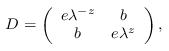
where b, z ∈ ℝ and e > 0 with e² = b² + 1. Create such an operator from parameters b and z.
operator_to_bz :: (Fractional a, Real a, RootTwoRing a) => Operator a -> (a, Double)Source
Conversely, given a positive definite real operator of
determinant 1, return the parameters (b, z). This is the
inverse of operator_from_bz. For efficiency reasons, the
parameter z, which is a logarithm, is modeled as a Double.
operator_to_bl2z :: (Floating a, Real a) => Operator a -> (a, a)Source
A version of operator_to_bz that returns (b, λ2z)
instead of (b, z).
This is a critical optimization, as this function is called often,
and logarithms are relatively expensive to compute.
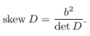
operator_skew :: Ring a => Operator a -> aSource
Compute the skew of a positive operator of determinant 1. We define the skew of a positive definite real operator D to be
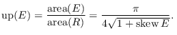
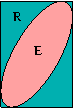
uprightness :: Floating a => Operator a -> aSource
Compute the uprightness of a positive operator D.
The uprightness of D is the ratio of the area of the ellipse E = {v | v†Dv ≤ 1} to the area of its bounding box R. It is given by
States
type OperatorPair a = (Operator a, Operator a)Source
A state is a pair (D, Δ) of real positive definite matrices of determinant 1. It encodes a pair of ellipses.
skew :: Ring a => OperatorPair a -> aSource
The skew of a state is the sum of the skews of the two operators.
bias :: (Fractional a, Real a, RootTwoRing a) => OperatorPair a -> DoubleSource
The bias of a state is ζ - z.
Grid operators
Consider the set ℤ[ω] ⊆ ℂ. In identifying ℂ with ℝ², we can alternatively identify ℤ[ω] with the set of all vectors (x, y)† ∈ ℝ² of the form
- x = a + a'/√2,
- y = b + b'/√2,
such that a, a', b, b' ∈ ℤ and a' ≡ b' (mod 2).
A grid operator is a linear operator G : ℝ² → ℝ² such that G maps ℤ[ω] to itself. We can characterize the grid operators as the operators of the form
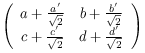
such that:
- a + b + c + d ≡ 0 (mod 2) and
- a' ≡ b' ≡ c' ≡ d' (mod 2).
A special grid operator is a grid operator of determinant ±1. All special grid operators are invertible, and the inverse is again a special grid operator.
Since all coordinates of ℤ[ω] (as a subset of ℝ²), and all entries of grid operators, can be represented as elements of the ring D[√2], the automorphism x ↦ x•, which maps a + b√2 to a - b√2 (for rational a and b), is well-defined for them.
In this section, we define some particular special grid operators that are used in the Step Lemma.
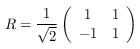
opR :: RootHalfRing r => Operator rSource
The special grid operator R: a clockwise rotation by 45°.
opA :: Ring r => Operator rSource
The special grid operator A: a clockwise shearing with offset 2, parallel to the x-axis.

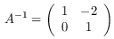
opA_inv :: Ring r => Operator rSource
The special grid operator A⁻¹: a counterclockwise shearing with offset 2, parallel to the x-axis.
opA_power :: RootTwoRing r => Integer -> Operator rSource
The operator Ak.
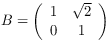
opB :: RootTwoRing r => Operator rSource
The special grid operator B: a clockwise shearing with offset √2, parallel to the x-axis.
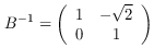
opB_inv :: RootTwoRing r => Operator rSource
The special grid operator B⁻¹: a counterclockwise shearing with offset √2, parallel to the x-axis.
opB_power :: RootTwoRing r => Integer -> Operator rSource
The operator Bk.
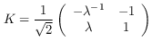
opK :: RootHalfRing r => Operator rSource
The special grid operator K.
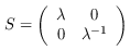
opS :: RootTwoRing r => Operator rSource
The special grid operator S: a scaling by λ = 1+√2 in the x-direction, and by λ⁻¹ = -1+√2 in the y-direction.
The operator S is not used in the paper, but we use it here for a more efficient implementation of large shifts. The point is that S is a grid operator, but shifts in increments of 4, whereas the Shift Lemma uses non-grid operators but shifts in increments of 2.
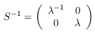
opS_inv :: RootTwoRing r => Operator rSource
The special grid operator S⁻¹, the inverse of opS.
opS_power :: RootTwoRing r => Integer -> Operator rSource
Return Sk.
Action of grid operators on states
action :: (RealFrac r, RootHalfRing r, Adjoint r) => (Operator r, Operator r) -> Operator DRootTwo -> (Operator r, Operator r)Source
Compute the right action of a grid operator G on a state (D, Δ). This is defined as:
(D, Δ) ⋅ G := (G†DG, G•TΔG•).
Shifts
A shift is not quite the application of a grid operator, because the shifts σ and τ actually involve a square root of λ. However, they can be used to define an operation on states.
shift_sigma :: RootTwoRing a => Integer -> Operator a -> Operator aSource
Given an operator D, compute σkDσk.
shift_tau :: RootTwoRing a => Integer -> Operator a -> Operator aSource
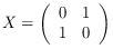
Given an operator Δ, compute τkΔτk.
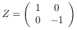
shift_state :: RootTwoRing a => Integer -> OperatorPair a -> OperatorPair aSource
Compute the k-shift of a state (D,Δ).
Skew reduction
lemma_A :: (RealFrac r, RootTwoRing r, Floating r) => r -> r -> IntegerSource
An implementation of the A-Lemma. Given z and ζ, compute the integer m such that the operator Am reduces the skew.
lemma_B :: (RealFrac r, RootTwoRing r, Floating r) => r -> r -> IntegerSource
An implementation of the B-Lemma. Given z and ζ, compute the integer m such that the operator Bm reduces the skew.
lemma_A_l2 :: (RealFrac r, RootTwoRing r, Floating r) => r -> r -> IntegerSource
A version of lemma_A that inputs λ2z instead of z and
λ2ζ instead of ζ. Compute the constant m such that the
operator Am reduces the skew.
lemma_B_l2 :: (RealFrac r, RootTwoRing r, Floating r) => r -> r -> IntegerSource
A version of lemma_B that inputs λ2z instead of z and
λ2ζ instead of ζ. Compute the constant m such that the
operator Bm reduces the skew.
step_lemma :: (RealFrac r, Floating r, Ord r, RootTwoRing r, RootHalfRing r, Adjoint r) => OperatorPair r -> Maybe (Operator DRootTwo)Source
An implementation of the Step Lemma. Input a state (D,Δ). If the skew is > 15, produce a special grid operator whose action reduces Skew(D,Δ) by at least 5%. If the skew is ≤ 15 and β ≥ 0 and z + ζ ≥ 0, do nothing. Otherwise, produce a special grid operator that ensures β ≥ 0 and z + ζ ≥ 0.
reduction :: (RealFrac r, Floating r, Ord r, RootTwoRing r, RootHalfRing r, Adjoint r) => OperatorPair r -> Operator DRootTwoSource
Repeatedly apply the Step Lemma to the given state, until the skew is 15 or less.
to_upright :: (RealFrac r, Floating r, Ord r, RootTwoRing r, RootHalfRing r, Adjoint r) => OperatorPair r -> Operator DRootTwoSource
Given a pair of ellipses, return a grid operator G such that
the uprightness of each ellipse is greater than 1/6. This is
essentially the same as reduction, except we do not assume that
the input operators have determinant 1.
to_upright_sets :: (Adjoint r, RootHalfRing r, RealFrac r, Floating r) => ConvexSet r -> ConvexSet r -> Operator DRootTwoSource
Given a pair of convex sets, return a grid operator G making both sets upright.
Action of special grid operators on convex sets
point_transform :: Ring r => Operator r -> Point r -> Point rSource
Apply a linear transformation G to a point p.
ellipse_transform :: (Ring r, Adjoint r) => Operator r -> Ellipse r -> Ellipse rSource
Apply a special linear transformation G to an ellipse A. This results in the new ellipse G(A) = { G(z) | z ∈ A }.
charfun_transform :: Operator DRootTwo -> CharFun -> CharFunSource
Apply a special grid operator G to a characteristic function.
lineintersector_transform :: Ring r => Operator DRootTwo -> LineIntersector r -> LineIntersector rSource
Apply a special linear transformation G to a line intersector. If the input line intersector was for a convex set A, then the output line intersector is for the set G(A) = { G(z) | z ∈ A }.
convex_transform :: (Ring r, Adjoint r, RootHalfRing r) => Operator DRootTwo -> ConvexSet r -> ConvexSet rSource
Apply a special linear transformation G to a convex set A. This results in the new convex set G(A) = { G(z) | z ∈ A }.
Bounding boxes
boundingbox_ellipse :: Floating r => Ellipse r -> ((r, r), (r, r))Source
Calculate the bounding box for an ellipse.
boundingbox :: Floating r => ConvexSet r -> ((r, r), (r, r))Source
Calculate a bounding box for a convex set. Returns ((x₀, x₁), (y₀, y₁)).
Auxiliary functions
within :: Ord a => a -> (a, a) -> BoolSource
We write x `within` (a,b) for a ≤ x ≤ b, or
equivalently, x ∈ [a, b].
fatten_interval :: Fractional a => (a, a) -> (a, a)Source
Given an interval, return a slightly bigger one.
lambda :: RootTwoRing r => rSource
The constant λ = 1 + √2.
lambda_inv :: RootTwoRing r => rSource
The constant λ⁻¹ = √2 - 1.
lambdapower :: RootTwoRing r => Integer -> rSource
Return λk, where k ∈ ℤ. This works in any RootTwoRing.
Note that we can't use ^, because it requires k ≥ 0, nor **,
because it requires the Floating class.
floorlog :: (Fractional b, Ord b) => b -> b -> (Integer, b)Source
logBase_double :: (Fractional a, Real a) => a -> a -> DoubleSource
special_inverse :: Ring r => Operator r -> Operator rSource
Calculute the inverse of an operator of determinant 1. Note: this does not work correctly for operators whose determinant is not 1.