hgg: A grammar of graphics plotting library for Haskell
The batteries-included entry point for hgg, a Haskell-native declarative
plotting library in the grammar-of-graphics tradition (ggplot2 /
Vega-Lite). Plots are built by monoid composition and can be bound to
dataframes by column name.
.
Depending on this package brings in the core (hgg-core), the dataframe
binding (hgg-frame) and the SVG backend (hgg-svg), and exposes a
single module Graphics.Hgg — one import Graphics.Hgg gives you the
Easy API, the full grammar API, the df |>> spec binding and SVG save
functions.
.
> import Graphics.Hgg
>
> main :: IO ()
> main = quickScatter "scatter.svg" [1,2,3,4,5] [1,4,9,16,25]
.
Optional backends are pulled in via manual cabal flags: pdf
(hgg-pdf), png (hgg-rasterific), latex (hgg-latex), 3d
(hgg-3d). Their modules (e.g. Graphics.Hgg.Backend.PDF) are imported
from the backend packages directly. Alternatively, depend on the backend
packages themselves — this umbrella is a convenience, not a requirement.
[Skip to Readme]


Flags
Manual Flags
| Name | Description | Default |
|---|---|---|
Pull in the PDF backend (hgg-pdf, needs a LaTeX engine at runtime) | Disabled | |
| png | Pull in the PNG backend (hgg-rasterific) | Disabled |
| latex | Pull in the LaTeX (TikZ) backend (hgg-latex) | Disabled |
| 3d | Pull in 3D plotting (hgg-3d) | Disabled |
Use -f <flag> to enable a flag, or -f -<flag> to disable that flag. More info
Downloads
- hgg-0.2.0.0.tar.gz [browse] (Cabal source package)
- Package description (as included in the package)
Maintainer's Corner
For package maintainers and hackage trustees
Candidates
- No Candidates
| Versions [RSS] | 0.1.0.0, 0.2.0.0 |
|---|---|
| Change log | CHANGELOG.md |
| Dependencies | base (>=4.17 && <5), hgg-core (==0.2.0.0), hgg-frame (==0.2.0.0), hgg-svg (==0.2.0.0) [details] |
| License | BSD-3-Clause |
| Copyright | 2026 Aelysce Project (Toshiaki Honda) |
| Author | Toshiaki Honda |
| Maintainer | frenzieddoll@gmail.com |
| Uploaded | by frenzieddoll at 2026-08-13T04:19:03Z |
| Category | Graphics |
| Home page | https://github.com/frenzieddoll/hgg |
| Distributions | Stackage:0.2.0.0 |
| Downloads | 24 total (7 in the last 30 days) |
| Rating | (no votes yet) [estimated by Bayesian average] |
| Your Rating | |
| Status | Docs available [build log] Last success reported on 2026-08-13 [all 1 reports] |
Readme for hgg-0.2.0.0
[back to package description]hgg — a grammar of graphics for Haskell
A Haskell-native declarative plotting library. Like ggplot2 and Vega-Lite it
follows the grammar of graphics philosophy: plots are built by monoid
composition — purePlot <> layer (mark …) <> settings …. It pairs with the
statistical library hanalyze
(hanalyze = analysis / hgg = visualization), so fitted models — regression, GLM,
GP, survival, time series, Bayesian HBM — can be overlaid directly onto plots.
Status: practical, pre-1.0 (API stabilising). SVG / PDF / PNG / Jupyter backends work today.
This is the umbrella package: depending on hgg brings in the core
(hgg-core), the dataframe binding (hgg-frame) and the SVG backend
(hgg-svg), and a single import Graphics.Hgg covers the whole default
experience.
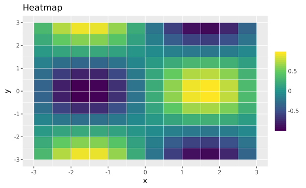
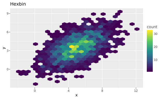
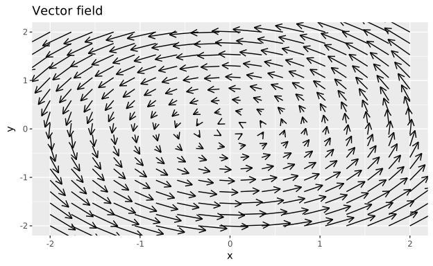
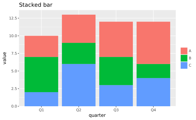
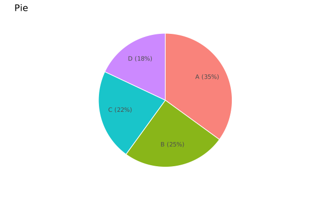
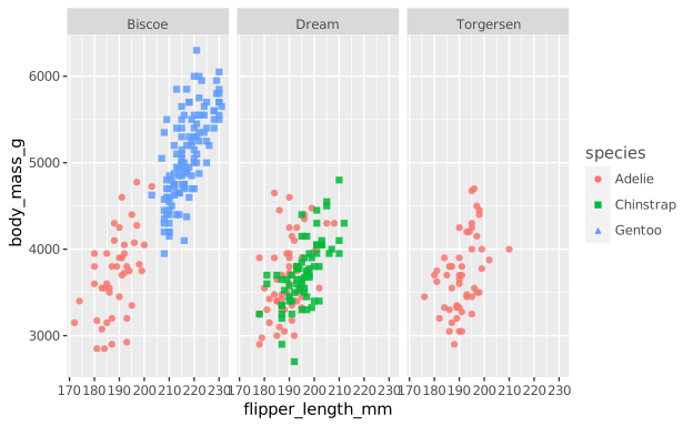
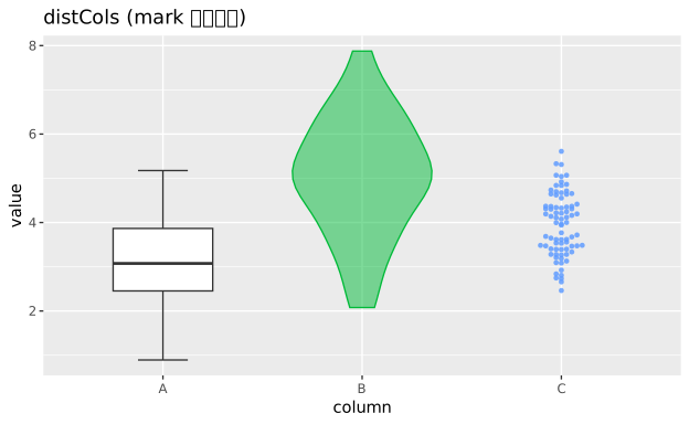
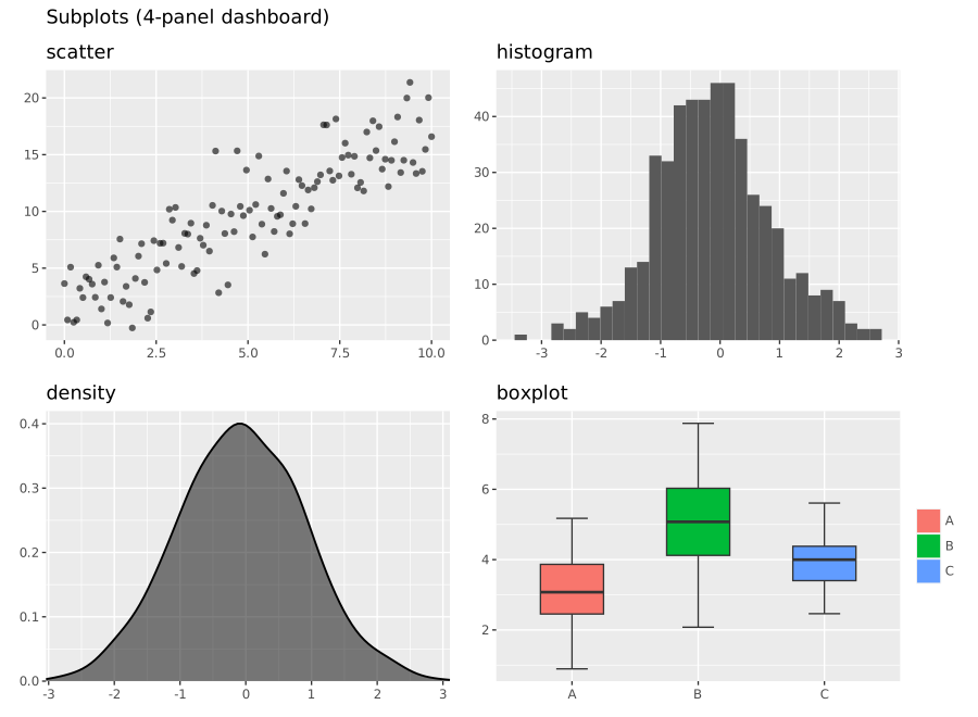
Gallery
 |
 |
 |
 |
 |
 |
 |
 |
 |
 |
 |
 |
 |
 |
 |
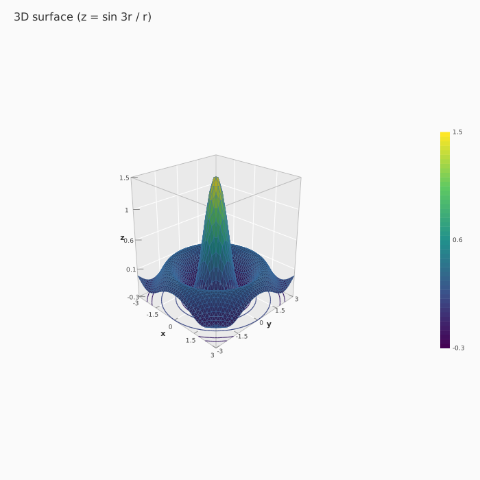 |
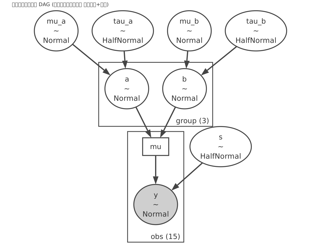 |
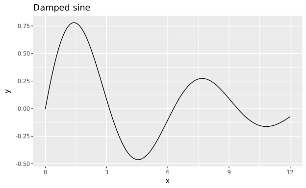
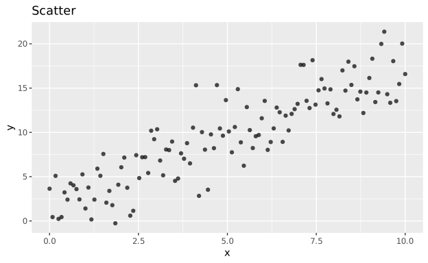
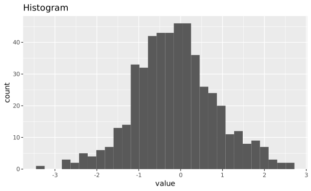
Click any figure to jump to its generating code
(hgg-tutorials/readme-images/ReadmeImages.hs);
the facet figure comes from the
R4DS tutorial.
The full API reference lives in the
api-guide.
All 24 penguins figures with reproduction code are in
R for Data Science, chapter 1.
Installation
Add hgg to your build-depends:
build-depends: hgg
Optional backends are enabled with manual cabal flags — in your
cabal.project:
constraints: hgg +pdf +png +latex +3d
| Flag | Pulls in | Gives you |
|---|---|---|
pdf |
hgg-pdf |
PDF output (Graphics.Hgg.Backend.PDF) |
png |
hgg-rasterific |
PNG output, Japanese fonts supported (Graphics.Hgg.Backend.Rasterific) |
latex |
hgg-latex |
LaTeX/TikZ output (Graphics.Hgg.Backend.LaTeX) |
3d |
hgg-3d |
3D plots, CPU projection (Graphics.Hgg.ThreeD) |
The umbrella is a convenience, not a requirement: you can instead depend on
the individual packages (hgg-svg, hgg-pdf, hgg-rasterific, hgg-latex,
hgg-3d, hgg-ihaskell, hgg-custom, hgg-analyze-bridge) and skip hgg
entirely — for Jupyter inline display use hgg-ihaskell.
Quick start
The shortest form is one line (one figure, no decisions beyond the data).
import Graphics.Hgg

main :: IO ()
main = quickScatter "scatter.svg" [1,2,3,4,5] [1,4,9,16,25]
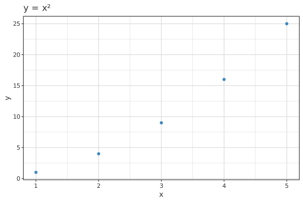
To add decorations, use the Easy helpers (direct values + overlay).
import Graphics.Hgg

main :: IO ()
main = saveSVG "easy.svg" $
     overlay [ points [1,2,3,4,5] [1,4,9,16,25] ]
  <> title "y = x²" <> xLabel "x" <> yLabel "y"
  <> widthUnit (600 *~ px) <> heightUnit (400 *~ px)
To work with column names, bind a data source with |>> (the idiomatic
style). Put a value that has columns on the left of |>> (below: inline
[(name, ColData)]) and refer to columns by name in the spec on the right.
|>> binds more loosely than <>, so no outer parentheses are needed even
with several layers.
import Graphics.Hgg
import qualified Data.Vector as V
import Data.Text (Text)

main :: IO ()
main = saveSVGBound "bound.svg" $
     cols |>> layer (scatter "x" "y")
  <> title "y = x²" <> xLabel "x" <> yLabel "y"
  where
    cols = [ ("x", NumData (V.fromList [1,2,3,4,5]))
           , ("y", NumData (V.fromList [1,4,9,16,25])) ] :: [(Text, ColData)]
A taste of the grammar
A plot is the empty purePlot plus layer (mark …) pieces combined with <>.
Data is bound with |>>; colour and shape are given inside the mark with
colorBy/shapeBy (below, raw is palmerpenguins).
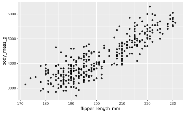
1. Scatter — a scatter mark with column names produces axes and points.
saveSVGBound "04-scatter.svg" $
  raw |>> layer (scatter "flipper_length_mm" "body_mass_g" <> alpha 0.85)
      <> xLabel "flipper_length_mm" <> yLabel "body_mass_g"
      <> theme ThemeGrey
2. Colour by species — add colorBy "species" to the mark.
saveSVGBound "05-color.svg" $
  raw |>> layer (scatter "flipper_length_mm" "body_mass_g"
                 <> colorBy "species" <> alpha 0.85)
      <> xLabel "flipper_length_mm" <> yLabel "body_mass_g"
      <> legendTitle "species"
      <> theme ThemeGrey
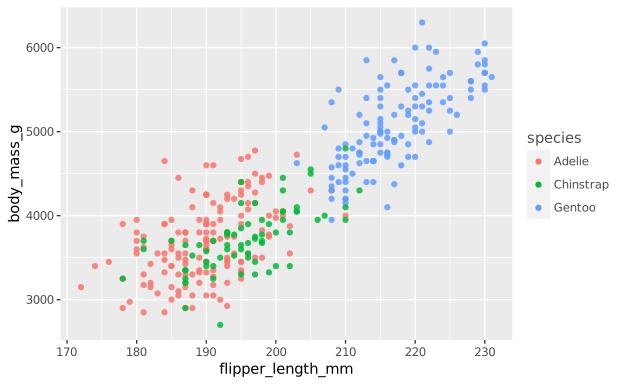
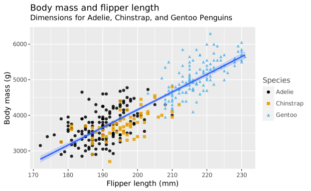
3. Overlay a regression line and labels — keep adding layers and decorations with <>.
saveSVGBoundStats "09-final.svg" $
  raw |>> layer (scatter "flipper_length_mm" "body_mass_g"
                 <> colorBy "species" <> shapeBy "species" <> alpha 0.85)
      <> layer (statLm "flipper_length_mm" "body_mass_g" <> color smoothBlue)
      <> palette okabeIto
      <> title "Body mass and flipper length"
      <> subtitle "Dimensions for Adelie, Chinstrap, and Gentoo Penguins"
      <> xLabel "Flipper length (mm)" <> yLabel "Body mass (g)"
      <> legendTitle "Species"
      <> theme ThemeGrey
The full step-by-step walkthrough is in the R for Data Science, chapter 1 tutorial.
What you can do
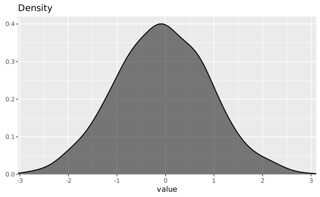
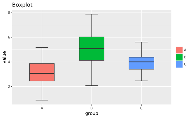
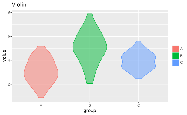
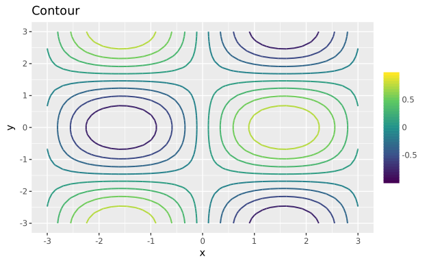
- Layer/mark declarative API — scatter, line, bar, histogram, boxplot, violin, density, band, forest, heatmap, contour, vector field, DAG, MCMC diagnostics, …
- DataFrame integration — write
df |>> layer (scatter "x" "y")with column names (NA rows are dropped automatically, i.e.na.rm) - Backends — SVG / PDF / PNG (Japanese fonts supported) / LaTeX (TikZ) / Jupyter (iHaskell) inline
- 3D — response surfaces (RSM) and generic 3D plots (CPU projection)
- Statistical integration —
toPlot/statLm/ HBM extractors draw hanalyze's fitted models directly - Full decoration set — themes / scales / facets / subplots / coordinate systems / reference lines / legends (ggplot-alike)
Documentation
- Gallery + full README
- API Reference — organised by topic
- Tutorial: R for Data Science, chapter 1
- Getting Started / ggplot2 Migration Guide
License
BSD-3-Clause (same as hanalyze).