| Copyright | (C) 2023 Alexey Tochin |
|---|---|
| License | BSD3 (see the file LICENSE) |
| Maintainer | Alexey Tochin <Alexey.Tochin@gmail.com> |
| Safe Haskell | None |
| Language | Haskell2010 |
| Extensions |
|
InfBackprop.Tutorial
Description
Tutorial inf-backprop package.
Synopsis
Quick start
>>>:set -XNoImplicitPrelude>>>import Prelude (Float, fmap)>>>import InfBackprop (BackpropFunc, call, derivative, derivativeN, pow)
We can define differentiable function
\[ f(x) := x^2 \]
as follows
>>>smoothF = pow 2 :: BackpropFunc Float Float
where pow is a power differentiable function and
BackpropFunc :: * -> * -> *
is a type for infinitely differentiable (smooth) functions.
We can get the function values by call method like
>>>f = call smoothF :: Float -> Float>>>fmap f [-3, -2, -1, 0, 1, 2, 3][9.0,4.0,1.0,0.0,1.0,4.0,9.0]
as well as the first derivative by derivative, which is
\[ f'(x) = 2 \cdot x \]
>>>df = derivative smoothF :: Float -> Float>>>fmap df [-3, -2, -1, 0, 1, 2, 3][-6.0,-4.0,-2.0,0.0,2.0,4.0,6.0]
or the second derivative
\[ f''(x) = 2 \]
>>>d2f = derivativeN 2 smoothF :: Float -> Float>>>fmap d2f [-3, -2, -1, 0, 1, 2, 3][2.0,2.0,2.0,2.0,2.0,2.0,2.0]
and so on.
A composition of two functions like
\[ g(x) := \log x^3 \]
must be defined with the categorical composition (>>>) (or (<<<))
>>>import InfBackprop (log)>>>import Control.Category ((>>>), (<<<))>>>smoothG = pow 3 >>> log
For more complicated expressions, for example,
\[ h(x) := x^2 + x^3 \]
we use arrow notations (***), first and second as follows
>>>import InfBackprop ((+), dup)>>>import Control.CatBifunctor ((***))
>>>smoothH = dup >>> (pow 2 *** pow 3) >>> (+) :: BackpropFunc Float Float
where
dup :: BackpropFunc a (a, a)
is differentiable function that simply splits the single implicit argument x into the tuple '(x, x)'.
THis is needed path tje implicit x to two independent functions pow 2 and pow 3.
The last
(+) :: BackpropFunc (a, a) a
operation transforms the pair of implicit arguments into their sum.
Derivatives for symbolic expressions
>>>import Prelude (($))>>>import Control.Category ((<<<))>>>import InfBackprop (BackpropFunc, call, derivative, derivativeN, sin, pow, (**), pow, setSecond, const)
We use simple-expr package here.
>>>import Debug.SimpleExpr.Expr (SimpleExpr, variable, simplify)
For example a symbolic function
\[ f(x) := \sin x^2 \]
can be defined as follows
>>>x = variable "x">>>f = sin <<< pow 2 :: BackpropFunc SimpleExpr SimpleExpr
see Tutorial for details.
We can call the symbolic function like
>>>call f xsin(x·x)
and find the symbolic derivative
\[ \frac{d}{d x} f(x) = \frac{d}{d x} \sin x^2 = 2\, x \cos x^2 \]
as follows
>>>simplify $ derivative f xcos(x·x)·(2·x)
as well as the second and higher derivatives
>>>simplify $ derivativeN 2 f x(((2·x)·-(sin(x·x)))·(2·x))+(2·cos(x·x))
Symbolic expressions visualization
The simple-expr package is equipped with a visulaisation tool that can be used to illustrate how the differentiation works.
>>>import Control.Category ((<<<))>>>import InfBackprop (call, backpropExpr)>>>import Debug.SimpleExpr.Expr (SimpleExpr, variable, simplify)>>>import Debug.SimpleExpr.GraphUtils (exprToGraph)>>>import Data.Graph.VisualizeAlternative (plotDGraph)
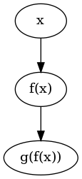
As a warm up consider a trivial composition of two functions
\[ g(f(x)) \]
is defined as
>>>x = variable "x">>>call (backpropExpr "g" <<< backpropExpr "f") xg(f(x))
It can be plotted by
plotExpr $ call (backpropExpr "g" <<< backpropExpr "f") x

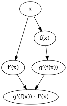
The graph for the first derivative can depicted by
plotExpr $ simplify $ derivative (backpropExpr "g" <<< backpropExpr "f") x

where
simplify :: SimpleExpr -> SimpleExpr
is a simple removal such things like *1 and +0.
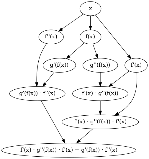
As well as the second derivative is straightforward
plotExpr $ simplify $ derivativeN 2 (backpropExpr "g" <<< backpropExpr "f") x

How it works
The idea would be clear from the example of three functions composition
\[
g(f(h(x)))
\]
with a focus on function f.
Its first derivative over x is
\[ g(f(h(x))). \]
\[ h'(x) \cdot f'(h(x)) \cdot g'(f(h(x))). \]
According to the backpropagation strategy, the order of the calculation should be as follows.
- Find
h(x). - Find
f(h(x)). - Find
g(f(h(x))). - Find the top derivative
g'(f(h(x))). - Find the next to the top derivative
f'(h(x)). - Multiply
g'(f(h(x)))onf'(h(x)). - Find the next derivative
h'(x). - Multiply the output of point 6 on
h'(x).
The generalization for longer composition is straightforward.
All calculations related to the function f can be divided into two parts.
We have to find f of h(x) first (forward step) and then the derivative f' of the same argument h(x) and
multiply it on the derivative g'(f(h(x))) obtained during the similar calculations for g (backward step).
Notice that the value of h(x) is reused on the backward step.
To implement this, we define type Backprop (see the corresponding
documentation for details).
Declaring custom derivative
>>>import Prelude (Float)>>>import qualified Prelude>>>import Control.Category ((>>>))>>>import InfBackprop ((*), negate, dup, BackpropFunc, Backprop(MkBackprop), second)
As an illustrative example a differentiable version of cos numerical function can be defined as follows
(see the documentation for Backprop for details)
  cos :: BackpropFunc Float Float
  cos = MkBackprop call' forward' backward' where
    call' :: Float -> Float
    call' = Prelude.cos

    forward' :: BackpropFunc Float (Float, Float)
    forward' = dup >>> first cos

    backward' :: BackpropFunc (Float, Float) Float
    backward' = second (sin >>> negate) >>> (*)

  sin :: BackpropFunc Float Float
  sin = ...
Here we use Prelude implementation for ordinary cos function in call.
The forward function is differentiable (which is needed for further derivatives) function
with two output values.
Roughly speaking forward is
x -> (sin x, x).
The first term of the tuple is just sin and
the second terms x in the tuple is the value to be reused on the backward step.
The backward is
(dy, x) -> dy * (-cos x),
where dy is the derivative found on the previous backward step and the second value is x stored by forward.
We simply multiply with (*) the derivative dy on the derivative of sin that is -cos.
The stored value is not necessary just x. It could be anything useful for the backward step, see for example
the implementation for exp and the corresponding
example
below.
Differentiation of monadic function
Differentiable versions of monadic functions a -> m b can also be backpropagated.
For example, consider a real-valued power function defined for positive real numbers.
For a negative number, it returns Nothing, which is a signal to stop computing the derivative and return Nothing
in the spirit of the behavior of the monad Maybe.
For this purpose, we can use that the type Backprop type is defined for any category,
not only for functions (->).
In particular, we can try Backprop(Kleisli Maybe) instead of Backprop(->) from the previous sections.
>>>import Prelude (Maybe, Maybe(Just, Nothing), ($), Ord, (>), Float)>>>import InfBackprop (Backprop(MkBackprop), derivative, dup, (*), linear, pureBackprop, first, second)>>>import Control.Arrow (Kleisli(Kleisli), runKleisli, (>>>))>>>import qualified NumHask as NH
The functoin
pureBackprop :: Monad m => Backprop (->) a b -> Backprop (Kleisli m) a b
is to trivially lift an ordinary backpropagation functions to the monadic function type.
Define the power function as follows
>>>:{powR :: forall a. (Ord a, NH.ExpField a) => a -> Backprop (Kleisli Maybe) a a powR p = MkBackprop call' forward' backward' where call' :: Kleisli Maybe a a call' = Kleisli $ \x -> if x > NH.zero then Just $ x NH.** p else Nothing -- forward' :: Backprop (Kleisli Maybe) a (a, a) forward' = pureBackprop dup >>> first (powR p) -- backward' :: Backprop (Kleisli Maybe) (a, a) a backward' = second der >>> pureBackprop (*) where der = powR (p NH.- NH.one) >>> pureBackprop (linear p) :}
and calculate
\[ \frac{d}{dx} x^{\frac12} = \frac{1}{2 \sqrt{x}} \]
for x=4 and x=-4 like
>>>runKleisli (derivative (powR 0.5)) (4 :: Float)Just 0.25>>>runKleisli (derivative (powR 0.5)) (-4 :: Float)Nothing
Differentiation with logging
Our objective now is to add logging to the derivative calculation.
The type Backprop cat a b type is parametrized by a category cat, input a and output b.
If cat is (->) the type is reduced to BackpropFunc we worked with above.
To add logging to the calculation we shall replace (->) by
MonadLogger m => Kleisli m.
We will need the imports below
>>>import Prelude (Integer, Float, ($), (+), (*))>>>import Control.Monad.Logger (runStdoutLoggingT, MonadLogger)>>>import Control.Arrow ((>>>), runKleisli, Kleisli)>>>import InfBackprop (derivative, loggingBackpropExpr)>>>import Debug.SimpleExpr.Expr (variable)>>>import Debug.LoggingBackprop (initUnaryFunc, initBinaryFunc, pureKleisli, exp, sin)
where the module loggingBackpropExpr contains some useful functionality.
For example, lifts for unary functions
initUnaryFunc :: (Show a, Show b, MonadLogger m) => String -> (a -> b) -> Kleisli m a b
and binary functions
initBinaryFunc :: (Show a, Show b, Show c, MonadLogger m) => String -> (a -> b -> c) -> Kleisli m (a, b) c
These two terms map given functions to Kleisli category terms, that allows logging during their execution.
Let us first explain how it works with the following example.
\[ f(x) = y \cdot 3 + y \cdot 4, \quad y = x + 2. \]
This function can be defined as follows
>>>:{fLogging :: MonadLogger m => Kleisli m Integer Integer fLogging = initUnaryFunc "+2" (+2) >>> (pureKleisli (\x -> (x, x))) >>> (initUnaryFunc "*3" (*3) *** initUnaryFunc "*4" (*4)) >>> initBinaryFunc "sum" (+) :}
We run the calculation with x = 5 as follows
>>>runStdoutLoggingT $ runKleisli fLogging 5[Info] Calculating +2 of 5 => 7 [Info] Calculating *3 of 7 => 21 [Info] Calculating *4 of 7 => 28 [Info] Calculating sum of 21 and 28 => 49 49
We are now ready to consider an example with derivatives. Let us calculate a simple example as follows
\[ \frac{d}{dx} \mathrm{f} (e^x) = e^x f'(e^x) \]
We define symbolic function f by
loggingBackpropExpr :: String -> BackpropFunc SimpleExpr SimpleExpr
and the entire derivative is
>>>runStdoutLoggingT $ runKleisli (derivative (exp >>> loggingBackpropExpr "f")) (variable "x")[Info] Calculating exp of x => exp(x) [Info] Calculating f of exp(x) => f(exp(x)) [Info] Calculating f' of exp(x) => f'(exp(x)) [Info] Calculating multiplication of 1 and f'(exp(x)) => 1·f'(exp(x)) [Info] Calculating multiplication of 1·f'(exp(x)) and exp(x) => (1·f'(exp(x)))·exp(x) (1·f'(exp(x)))·exp(x)
For illustration we can set 'f = sin' and 'x=2'
\[ \left. \frac{d}{dx} \sin (e^x) \right|_{x=2} = e^2 \cos (e^2) \]
>>>runStdoutLoggingT $ runKleisli (derivative (exp >>> sin)) (2 :: Float)[Info] Calculating exp of 2.0 => 7.389056 [Info] Calculating sin of 7.389056 => 0.893855 [Info] Calculating cos of 7.389056 => 0.44835615 [Info] Calculating multiplication of 1.0 and 0.44835615 => 0.44835615 [Info] Calculating multiplication of 0.44835615 and 7.389056 => 3.312929 3.312929
The first thing to mention in these logs is that the last forward step
sin(exp x)
is still computed, unlike the examples from the previous section.
This is due to the monadic nature of the calculation chain, that must disappear as soon as we return to
(->) from Kleisli m.
The second thing to mention here is that the exponent
exp x
is calculated only once thanks to the cache term passed from the forward to the backward method.